I was away walking the West Highland Way this last week - beautiful.
But “I” (my pc and claude) did some of my best TRPT optimisation work while I was walking
Attached is the report
TRPT_AWE_Forum_Report_v3.docx (2.0 MB)
Disappointingly the v4 ring spacing optimisation diagram in the report seems to show rings equally spaced along the shaft , which is entirely not the point of what was learned or observed… should be rebuilt from the data when I get another bot with enough credit to churn through
1 Like
OK the latest optimisation found that 8 lines gives a lighter system.
Looks like we’re going to want very skinny blades in that case to lower solidity.
Arrrgh so many factors / parameters
but it makes very pretty colourful simulations
I’ll push some new GitHubs later
there’s a new set of analysis tools for non geeks to follow soon.
The numbers are too dense to read as is… must make the dash more human
OK we have now got a dynamic “furl” simulated
The backline release to lift and pitch the rotor
There are still some tweaks to do - I’m very suspicious of how fast that power falls out of the rotor
You know anyone who likes the kite power simulation stuff and wants to kick the tyres?
tell them Rod sent you
Hadn’t settled enough before the “furl” and there was no easing to release the backline…
Looking a lot more like it… I’m manually dragging the timeline scroller so it’s still a little jumpy
1 Like
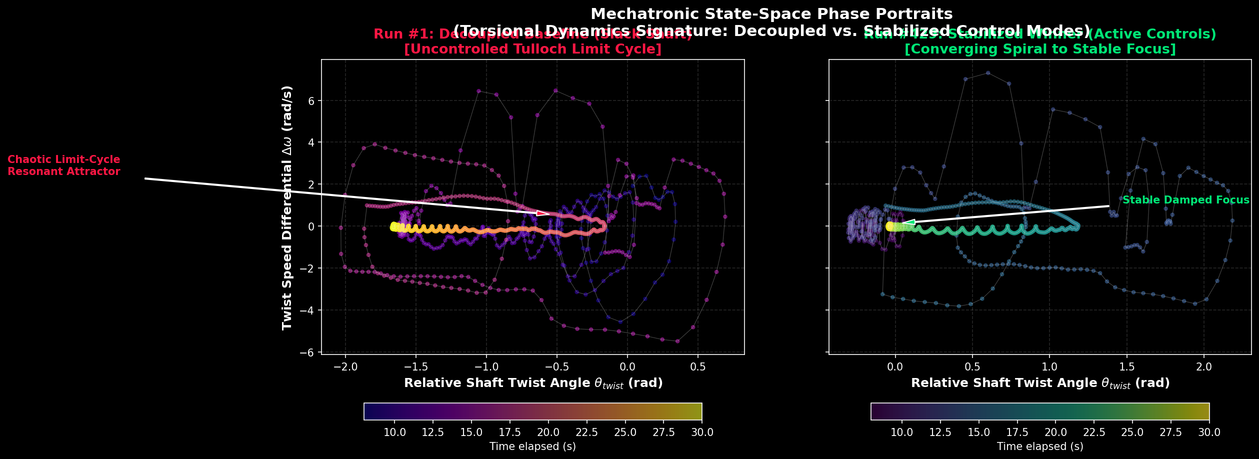
Still got a bit of whack-a-mole to play with the code but
It’s getting more reliable and realistic every day
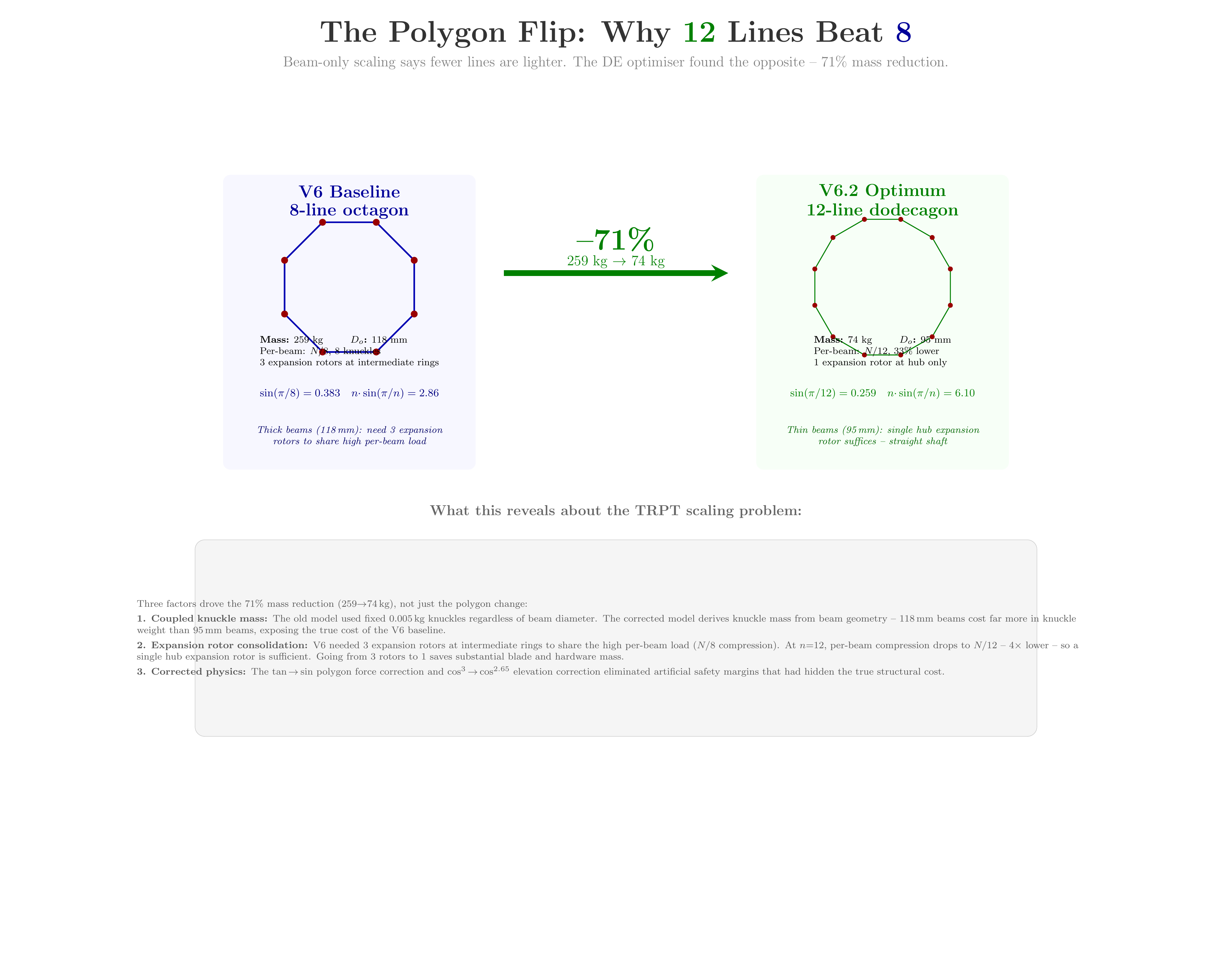
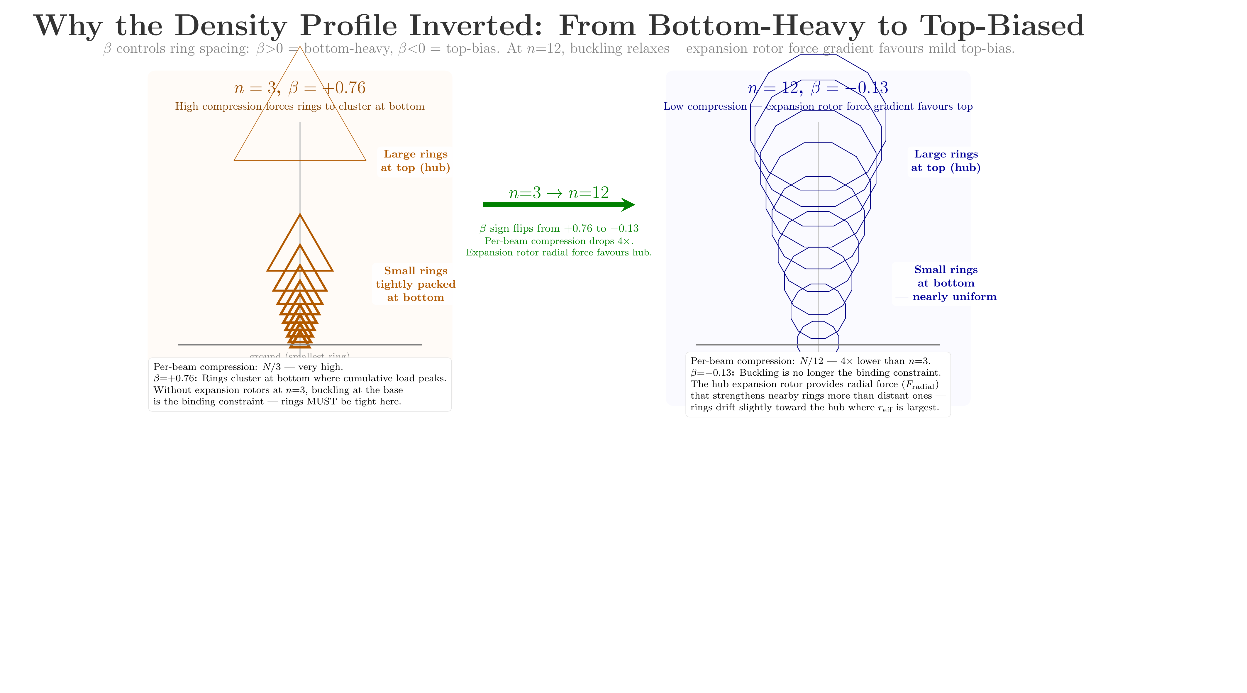
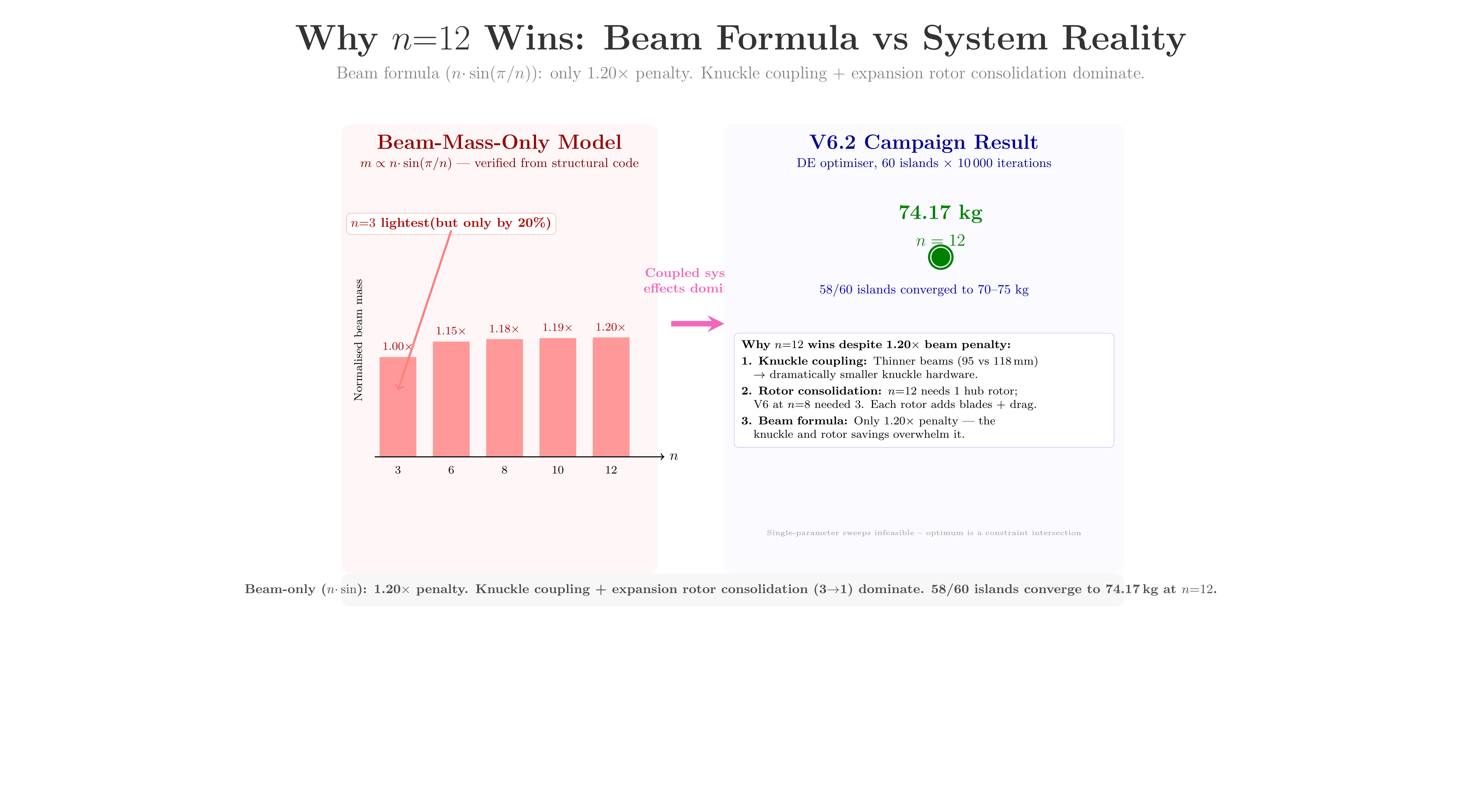
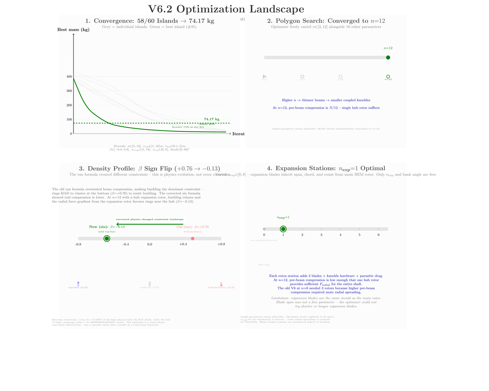
Looks like I have to run a v6_3 if that statement about there being only 3 blades added in an expansion rotor to a 12 blade system is true… It’s Simple mistakes like that…
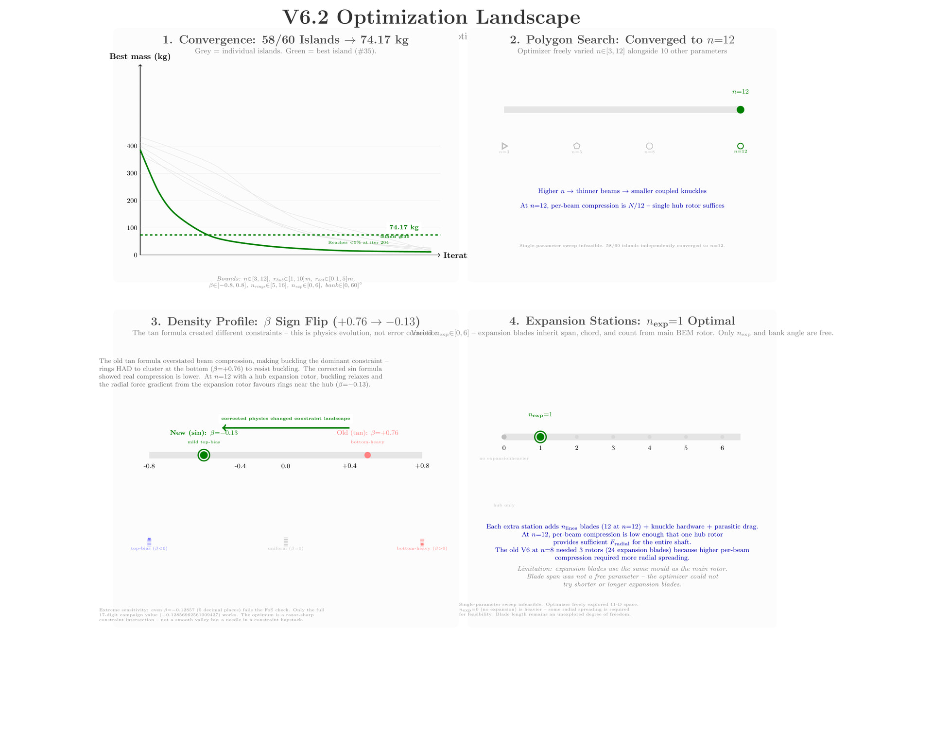
Oh good news, the mistake was in the diagram generation code
Improved
Ok
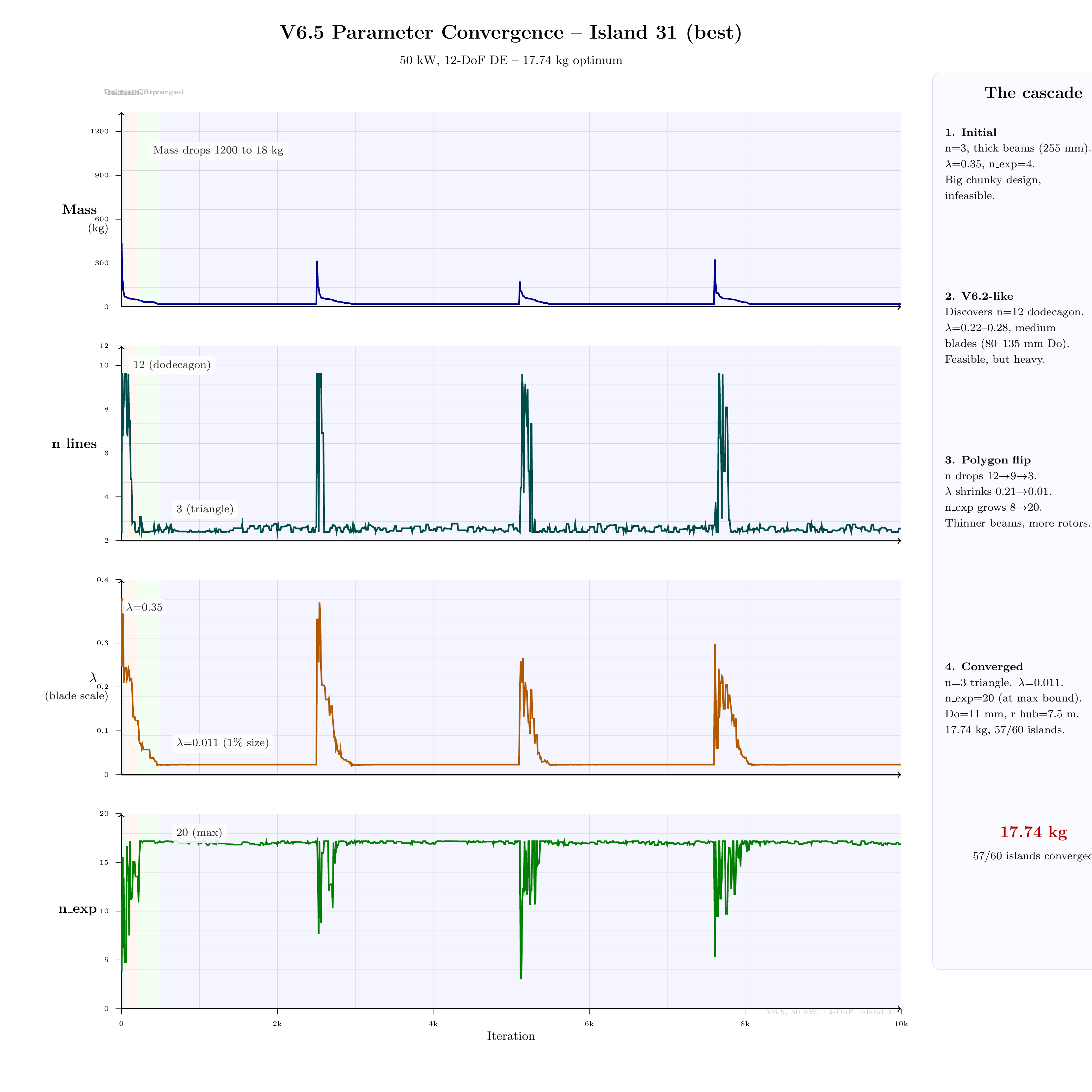
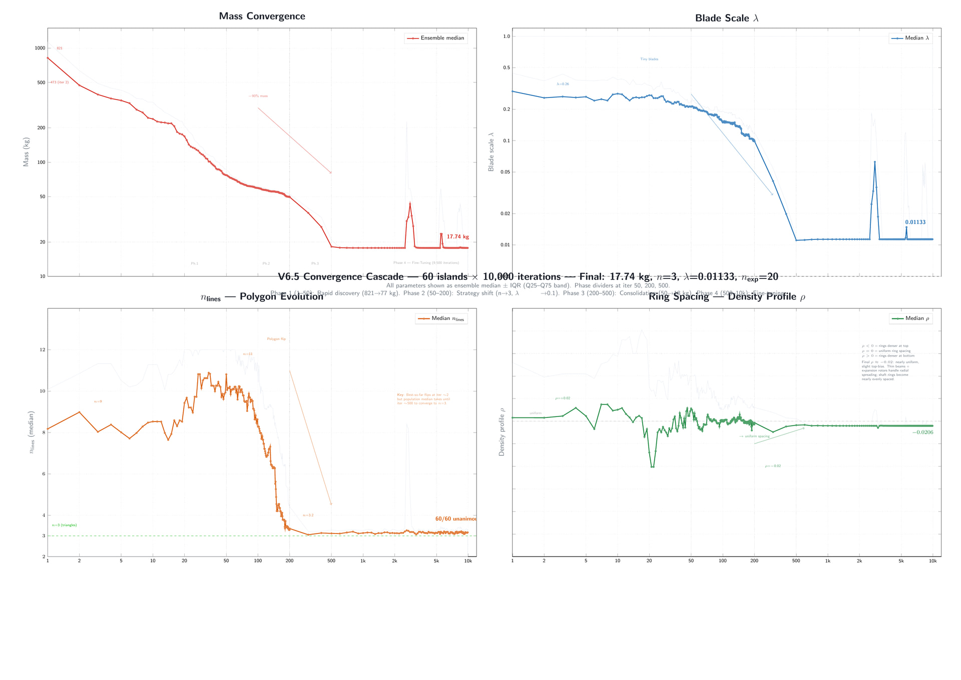
More parameters and options in the search… it flipped back to 3 beams, triangle TRPT.
Urgghhhh another mole to whack
mach 0.6 is total nonsense
Please ignore the robots design once again
It ignored 32MW of drag at that wonderful speed
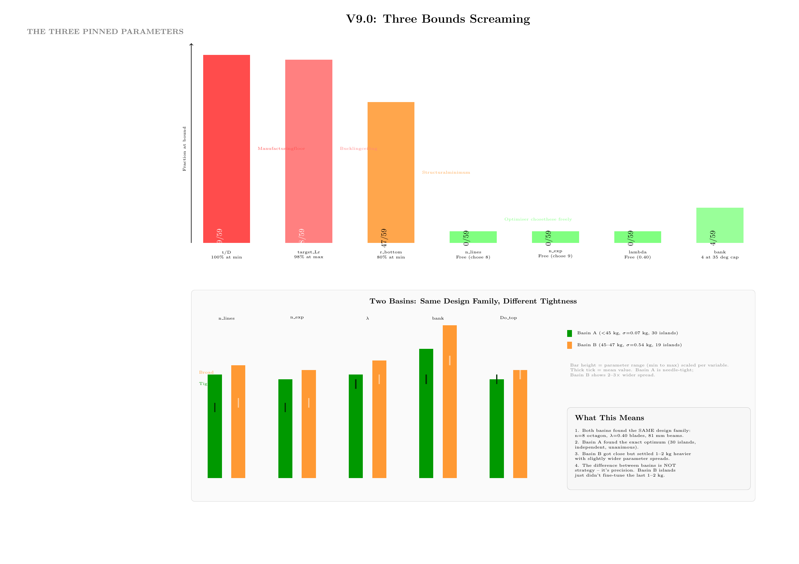
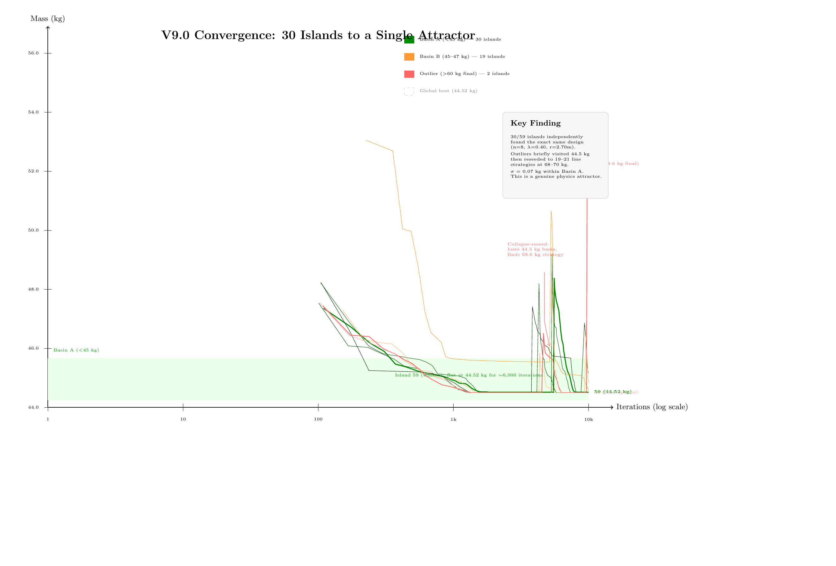
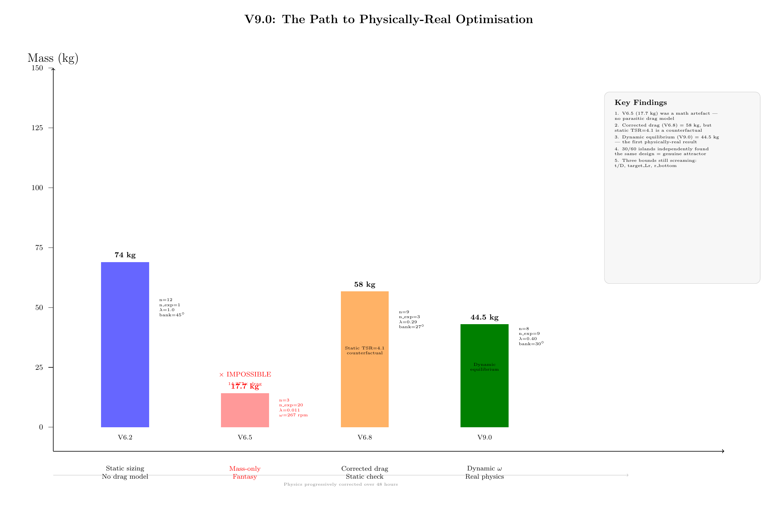
Turns out it hadn’t been running on a settled running model, just an estimation.
Can’t trust these models not to meddle and reconfigure for efficiency , unless they have super tight spec boundaries
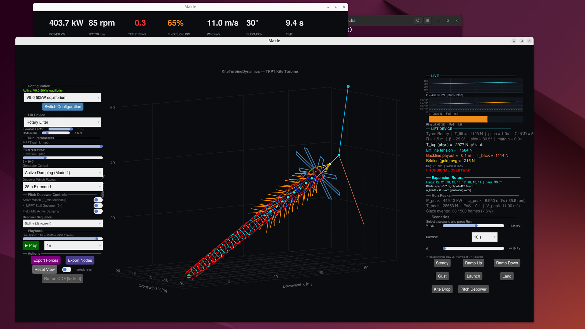
Waaay out of spec
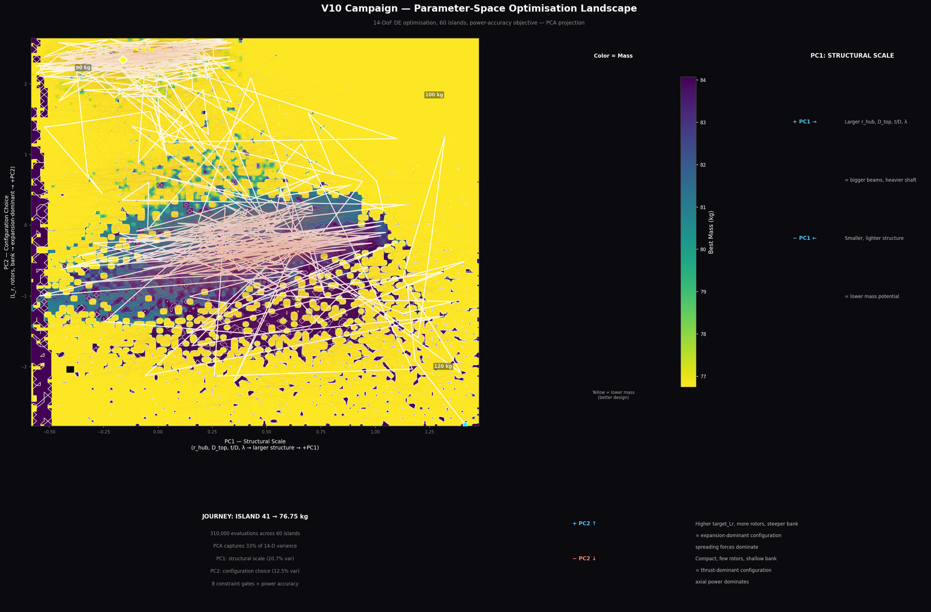
The landscape shows the V10 campaign’s parameter space at a glance:
- Yellow valley (top-left): the optimum at 76.75 kg — where the white trajectory ends
- Purple peaks (center-right): high-mass regions the optimizer avoided
- Contour lines: thin white lines tracing the mass topography at 78, 80, 82, 84, 90, 100 kg
- 60 spiderweb trajectories (faint pink): every island’s exploration path
- Island 41 path (white, labeled): cyan start → yellow diamond finish
- PC interpretation panels: what the axes mean physically
- 310K evaluations, 33% PCA variance captured
A dark-themed scientific visualization showing the V10 campaign’s parameter-space optimisation landscape. A 2D PCA projection of 310,000 evaluations across 60 islands reveals a yellow valley (low mass, ~77 kg) in the top-left where the optimum design sits, and purple peaks (high mass, 84+ kg) in the center-right where the optimizer avoided. Thin white contour lines trace the mass topography at 78, 80, 82, 84, 90, and 100 kg. A white trajectory line traces Island 41’s convergence path from a cyan start marker to a yellow diamond end marker at 76.75 kg. Faint pink spiderweb lines show the exploration paths of all 60 islands. Right-side panels explain that PC1 (x-axis) represents structural scale — larger hubs and beams to the right — while PC2 (y-axis) represents configuration choice — more rotors and steeper bank upward. A vertical colorbar maps yellow through green to purple from 77 to 84 kg. Bottom text notes 310,000 total evaluations with PCA capturing 33% of the 14-dimensional variance.
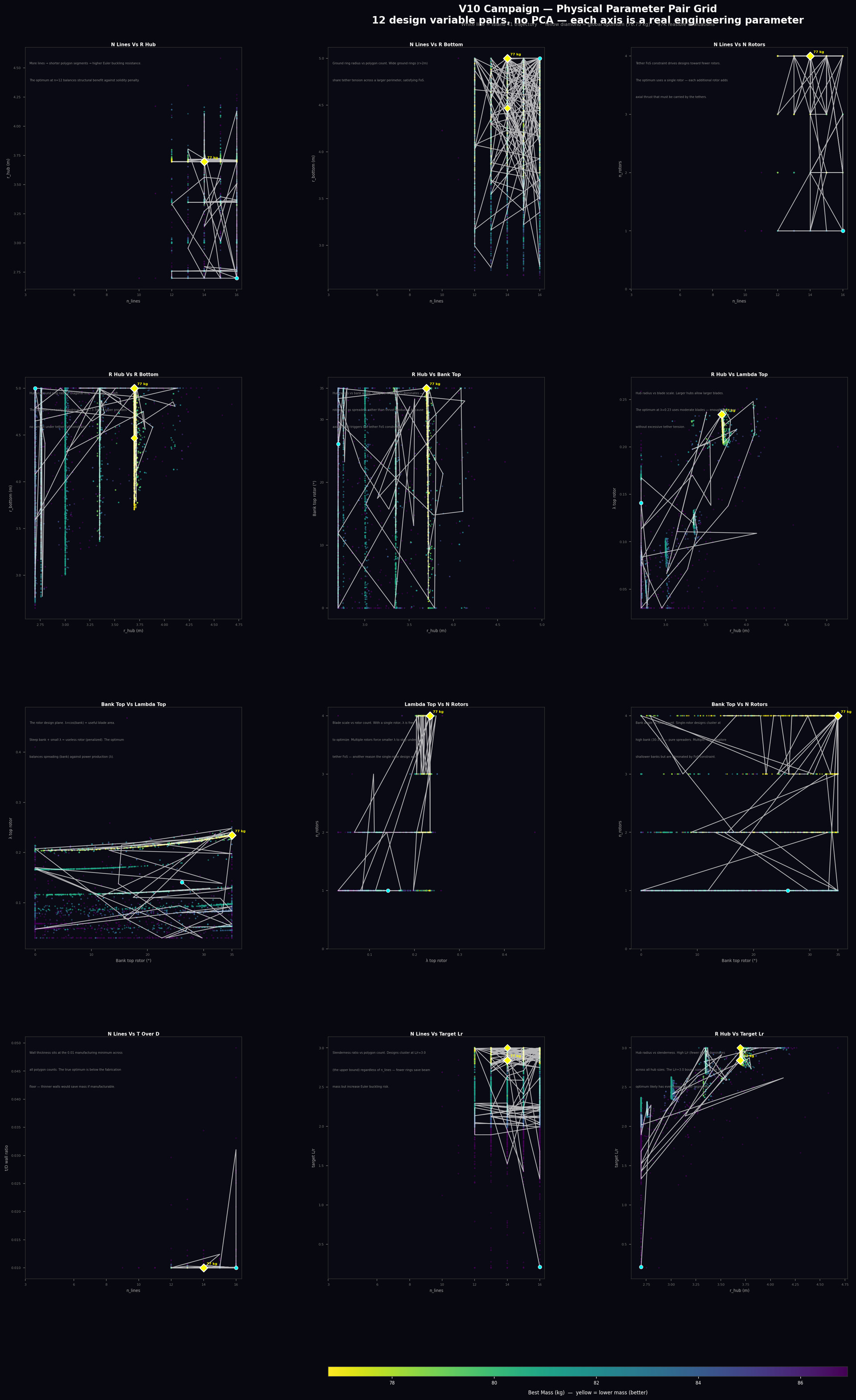
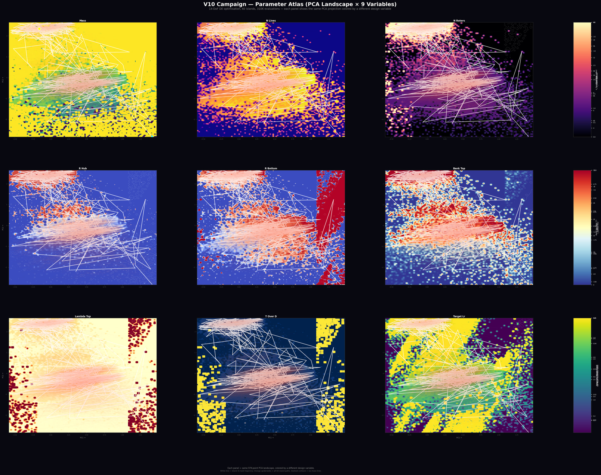
Well, with a parameter pairs map and a parameter atlas , you should be able to go build one of these 50kW monsters
V10 Campaign — Traced Performance Paths Over Non-Dimensional Contour Space
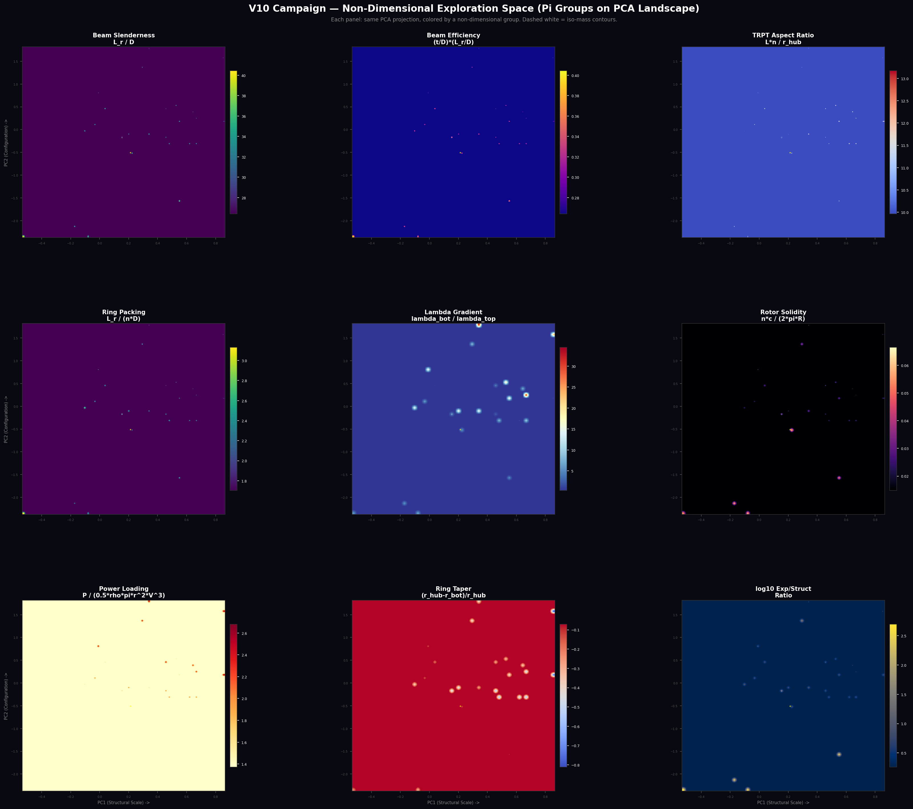
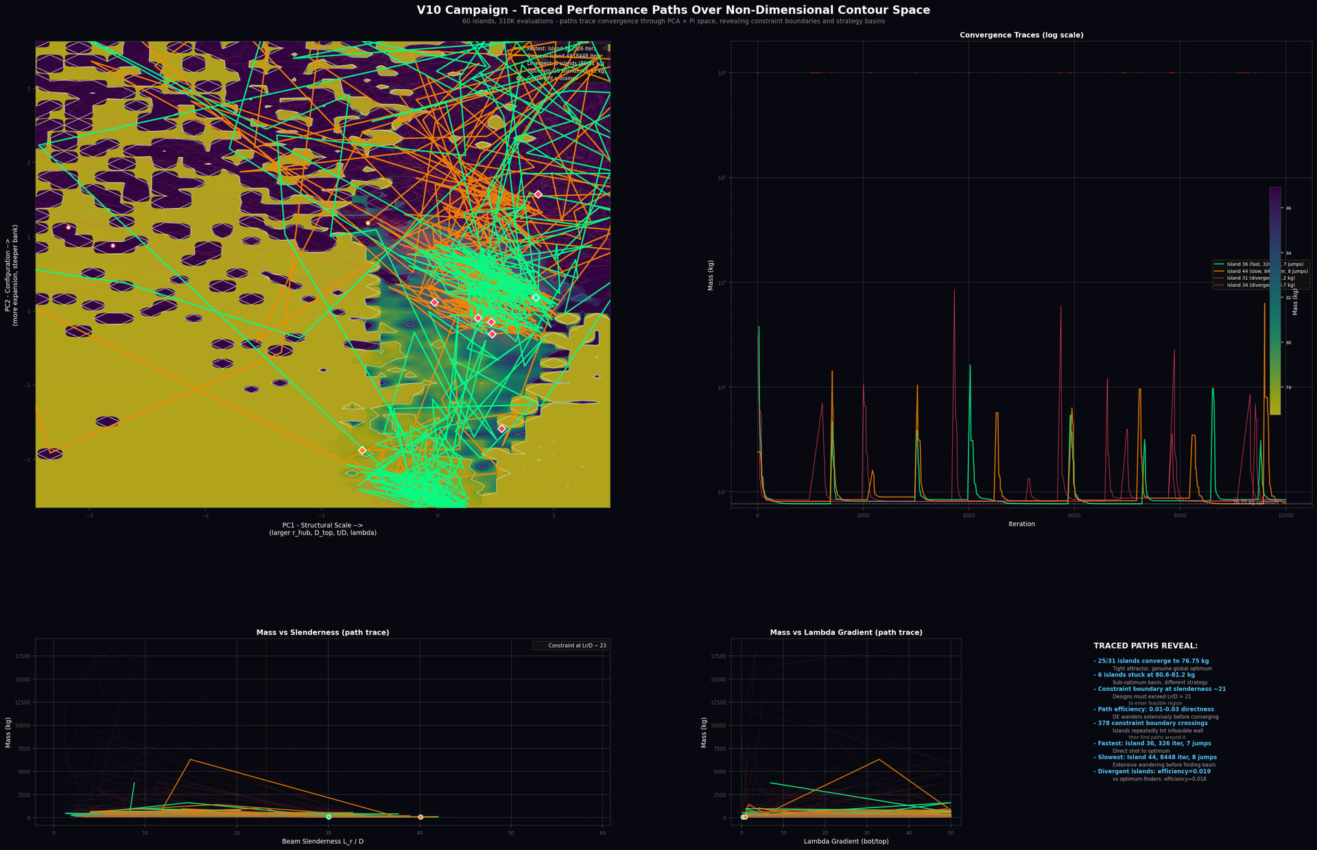
Accompanying diagram: v10-traced-paths.png
Source campaign: V10, 60 islands, 310,000 evaluations, 14-DoF DE optimisation
Best design: Island 41, 76.75 kg, 12-line dodecagon, 1 rotor, 35° bank
What this diagram shows
A four-panel figure that traces the convergence of 31 differential evolution
islands through the same PCA-projected parameter space used in the non-
dimensional atlas. While the atlas shows static snapshots coloured by Pi
groups, this diagram shows the dynamic paths — how each island moved through
the space, where it hit constraints, and how quickly it found the optimum.
Panel layout:
Top-left PC landscape with density background, iso-mass contours,
all 31 island trajectories overlaid, and constraint boundary
crossing points marked.
Top-right Mass vs iteration on a semi-log scale for key islands,
showing convergence speed and constraint-wall encounters.
Bottom-left Mass vs beam slenderness (L_r/D) for all island paths,
revealing the constraint gate and descent corridor.
Bottom-middle Mass vs lambda gradient (bot/top) for all island paths,
showing the basin-selection threshold.
Bottom-right Summary findings as text.
Trajectory colour coding
Green — Fastest optimum-finder (Island 36, 326 iterations to 5% of optimum)
Orange — Slowest optimum-finder (Island 44, 8,448 iterations)
Red — Divergent islands that never found the optimum (6 islands, 80-81 kg)
Cyan — All remaining optimum-finders (25 islands total)
White diamonds mark the start of each highlighted trajectory; coloured
diamonds mark the final converged position.
The constraint boundary
Red scatter points in the top-left panel mark every location where an island
crossed the feasibility threshold — either entering the feasible region from
the infeasible wall, or being thrown back out after a reseed. A total of 378
crossing events were recorded across 31 islands (mean ~12 per island).
The boundary sits at beam slenderness L_r/D ≈ 21. Below this value, parasitic
drag on the structural elements exceeds the total aerodynamic power available
from all rotors — the design is an air brake, not a turbine. Every island
that reached the optimum first had to discover and cross this gate.
The boundary is visible as a vertical dashed red line in the bottom-left
panel (Mass vs Slenderness). Paths that approach from the left are in the
infeasible region; crossing to the right enters feasibility. The optimum
sits at L_r/D ≈ 39 — nearly twice the threshold — because mass continues
to decrease with slenderness until the design bounds are reached.
The two-basin architecture
The PC landscape reveals two distinct attractors separated by a fitness
barrier:
Basin A (76.75 kg) — 25/31 islands
PC1 ≈ 0.0, PC2 ≈ −2.0
Slenderness ≈ 39, λ gradient ≈ 4-5
Expansion-dominant, structurally lean. The global optimum.
Basin B (80.6-81.2 kg) — 6/31 islands
PC1 ≈ +0.5, PC2 ≈ −0.5
Slenderness ≈ 25-35, λ gradient ≈ 8-15
Moderately lean but poor expansion/thrust balance. A local optimum.
Islands in Basin B never discover Basin A because the path between them
passes through higher-mass (100-150 kg) intermediate designs that the DE’s
selection pressure rejects. The basins are separated in Pi-space primarily
by lambda gradient — Basin A designs reduce bottom-blade overshoot to ~4×,
while Basin B designs remain at 8-15×.
This is visible in the bottom-middle panel (Mass vs Lambda Gradient): the
green and orange paths descend below λ_grad ≈ 7 en route to the optimum,
while the red paths plateau at higher gradients and settle at 80-81 kg.
Convergence behaviour
The convergence traces in the top-right panel reveal the temporal structure:
-
All islands start at high mass (200-10,000 kg or infeasible) and
descend rapidly in the first ~500 iterations as they discover the
feasible region. -
Spikes back to ~1,000,000 kg are reseed events — the DE population
collapses, is re-initialised randomly, and must rediscover feasibility.
The fastest island (36) had 4 reseeds; the slowest (44) had 8. -
After the final reseed, convergence to the basin floor is rapid —
typically 200-500 iterations from first feasible entry to within 5%
of the final mass. -
The divergent islands (red) show a different pattern: they enter the
feasible region early, descend to 80-81 kg, and then flatline. They
never reseed out of Basin B because the DE population has converged
within that local attractor.
Path efficiency
The path directness metric (Euclidean start-to-end distance divided by total
path length) quantifies exploration cost:
All optimum-finders: 1.7% ± 0.8% efficient
Divergent islands: 1.6% ± 0.5% efficient
Fastest (Island 36): 3.1% efficient
Slowest (Island 44): 1.1% efficient
The DE spends 96-99% of its movement budget on exploration — probing
constraint boundaries, recovering from reseeds, mapping the feasible
region’s shape. The “fast” islands are not smarter; they simply started in
regions of PC space with clearer gradient toward the Basin A entrance.
The performance signature
Three Pi-space trajectories define the outcome classes:
Fast optimum: Rapid slenderness climb → crosses L_r/D > 21 early →
λ gradient drops below 7 → direct descent to 76.75 kg.
Islands 36, 45, 49.
Slow optimum: Extended wandering along constraint wall → many boundary
hits → eventually finds feasible corridor → same descent
to 76.75 kg. Islands 43, 44.
Divergent: Achieves slenderness > 21 → enters feasible region →
λ gradient stalls at 8-15 → settles at 80-81 kg, never
discovers the lower basin. Islands 31, 34, 37, 42, 50, 53.
The divergent islands all share the same failure mode: they clear the
structural feasibility gate (slenderness) but never find the configuration
gate (λ gradient). This confirms that the exploration space has a two-stage
performance filter.
What this means for the design space
-
The global optimum at 76.75 kg is a genuine, tight attractor — 25
independent DE islands from different random starts all found exactly
the same basin. This is strong evidence that the result is not a fluke
of the optimiser. -
The exploration space is shaped by two non-dimensional gates: a hard
structural feasibility threshold (L_r/D > 21) and a softer configuration
threshold (λ_bot/λ_top < 7). Designs that clear only the first gate
settle at ~15% higher mass. -
The constraint boundary (378 crossings) is the dominant feature of the
landscape. Future campaigns with wider bounds should expect even more
boundary interaction as the DE probes further into the infeasible region. -
Path efficiency of ~2% is typical for DE on this landscape and should
be budgeted for in campaign planning. A 10,000-iteration island run
is not “slow” — it is the expected cost of adequate exploration. -
The three bound-screaming parameters (t/D, L_r, r_bottom) are all on the
structural slenderness axis. The next campaign that widens these bounds
should expect the optimum to shift leftward in PC1 (structurally leaner)
with the same PC2 (configuration) — confirming that structural leanness
and configuration balance are genuinely separable optimisation sub-
problems.
But of course as hopeful as that all sounded
it fails when it meets the dynamics dashboard
OH - Scratch that
It was a generator mismatch - oh maybe not
No in the capability of the k_mppt to crossover with the turbine operating point…
No… yet again…
It was rotor settling with wrong rotor numbers and positions logic making a loose line scenario which crashed the generation capacity
You need a lot of patience for these superpowers
Or
You just need to upgrade the superpowers

I’ve been using classic RAG for too long (I’m at least 10 days behind this now) 
And while that was loading on the laptop…
A few corrections, investigations, and
The regeneration of a more likely optimal Kite Turbine
but 13 lines… eugh- yuck
Loads more images available on the KiteTurbineDynamics.jl/docs/awes-forum-diagrams at master · rodWindswept/KiteTurbineDynamics.jl · GitHub
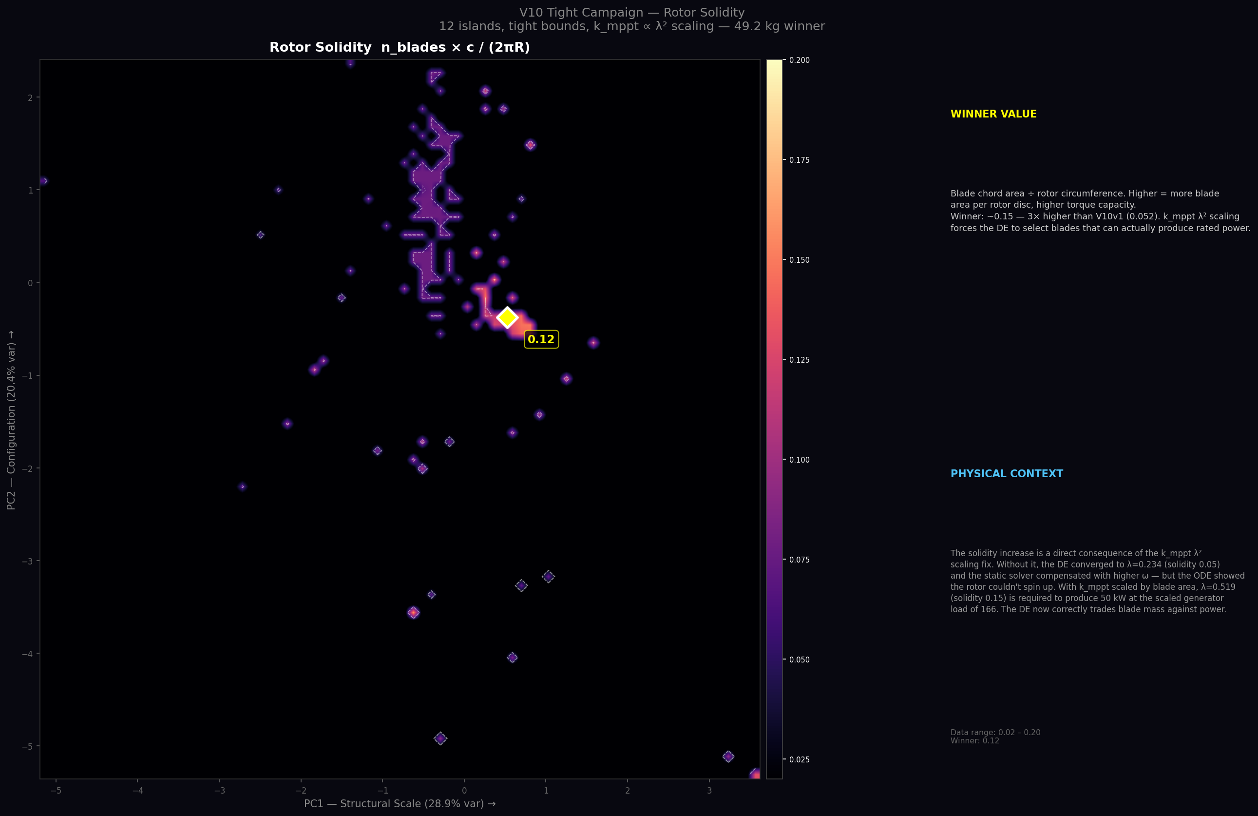
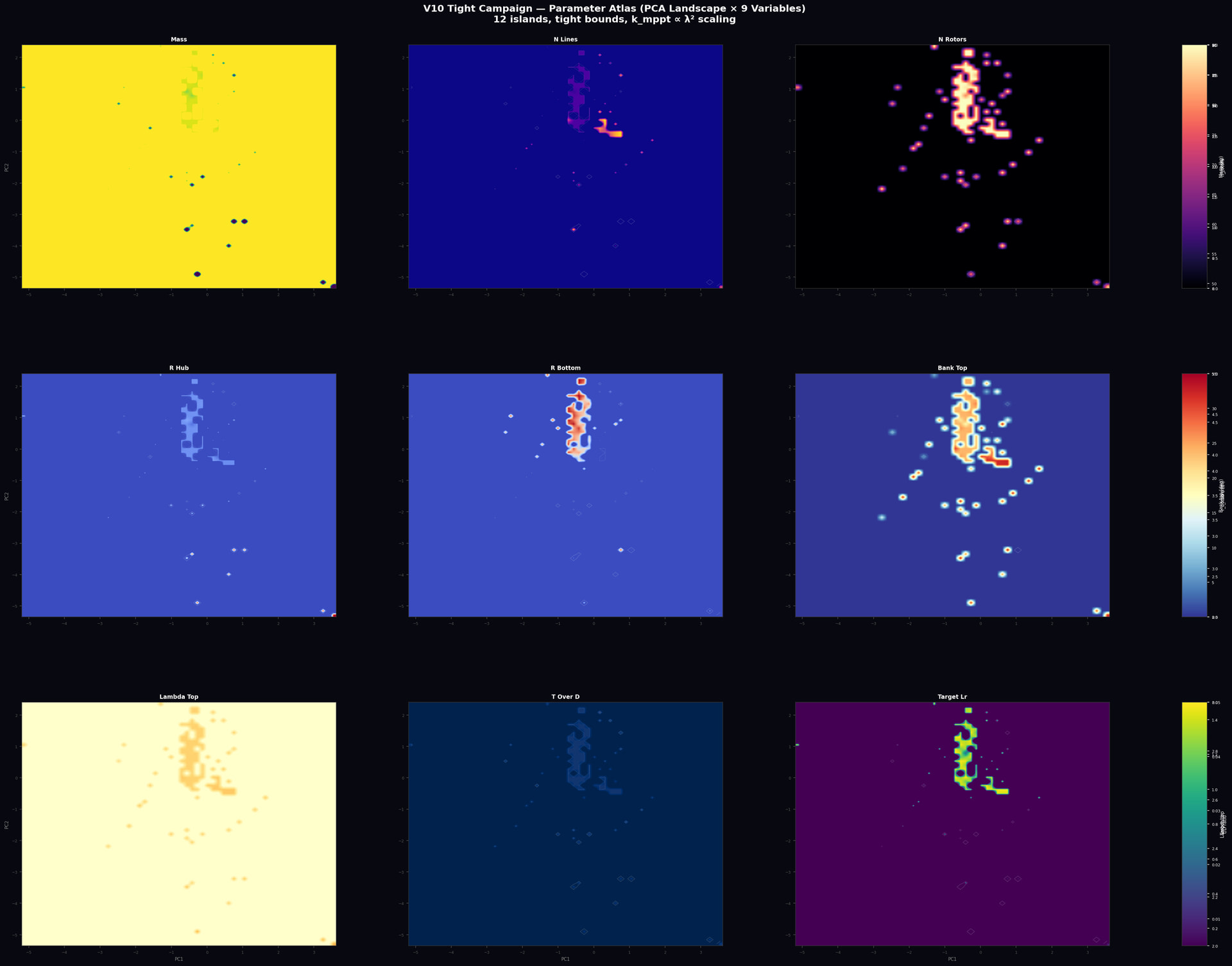
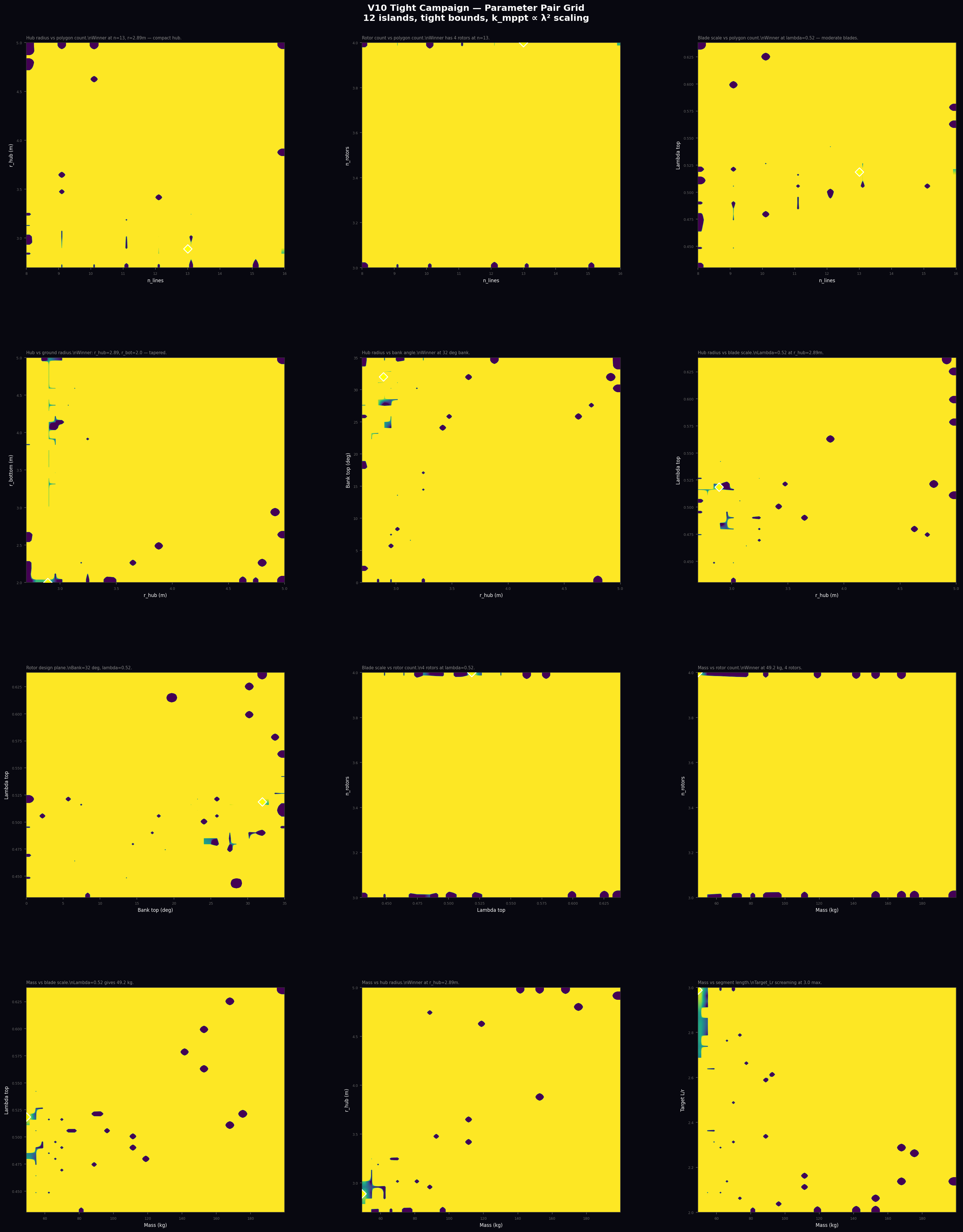
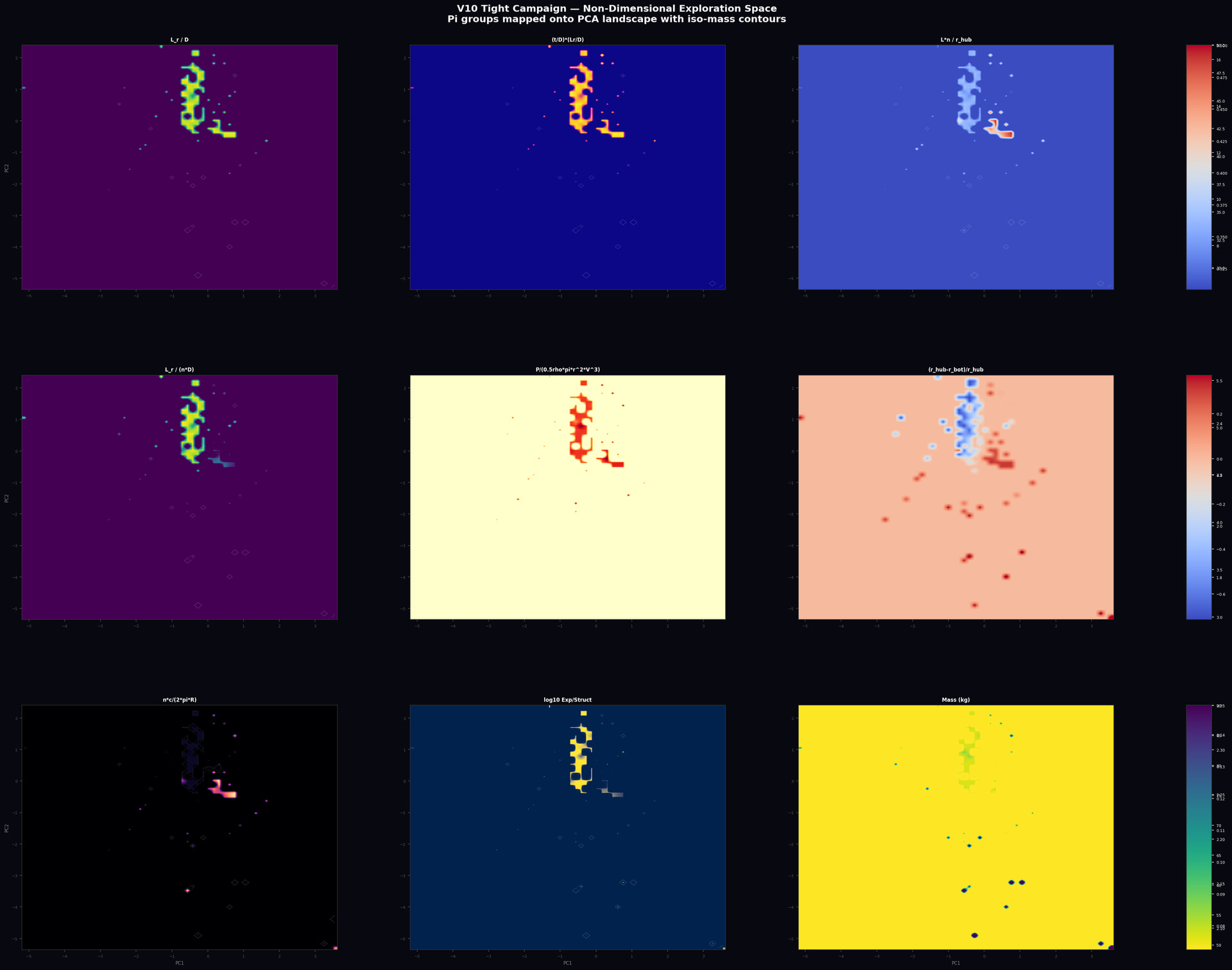
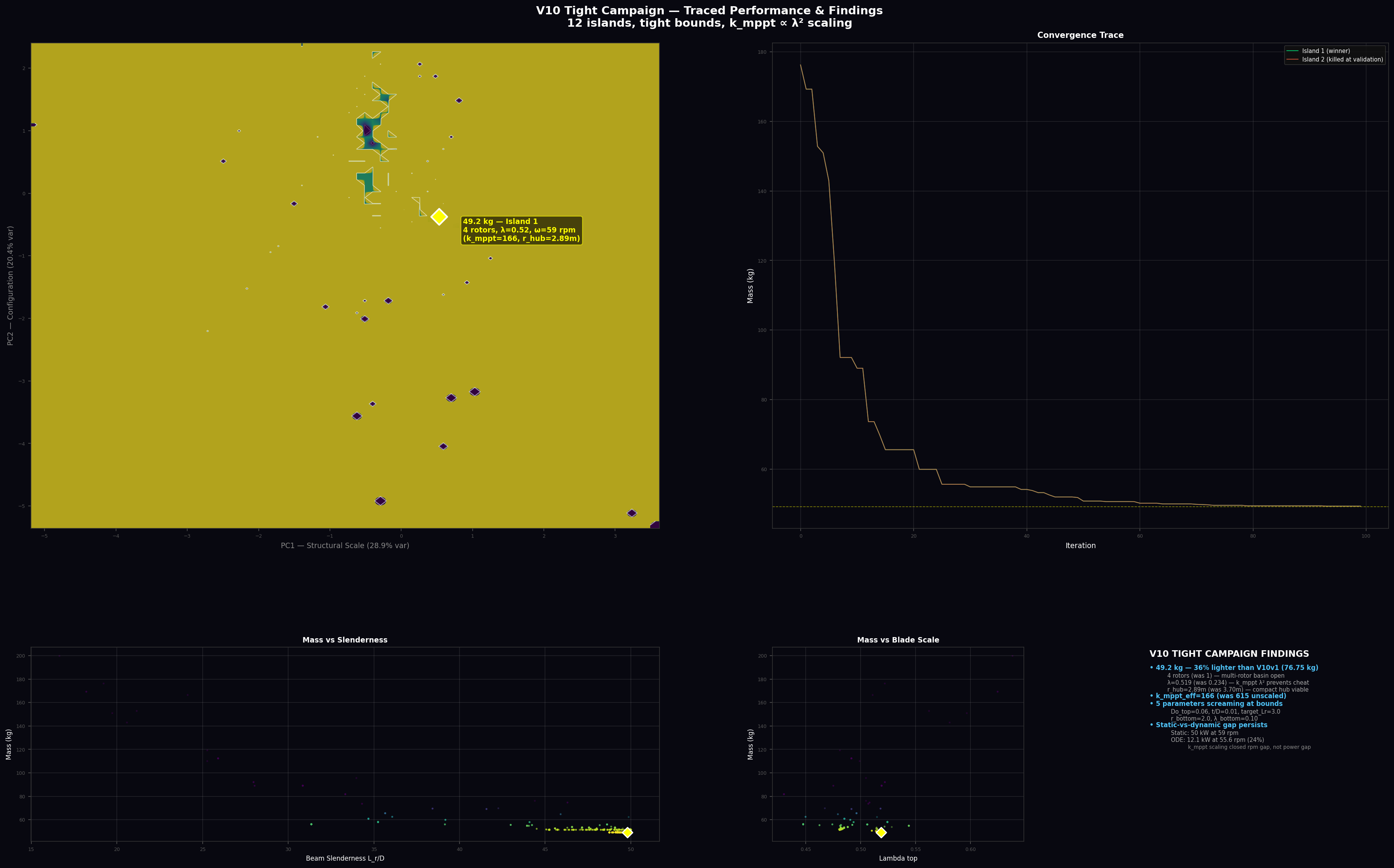
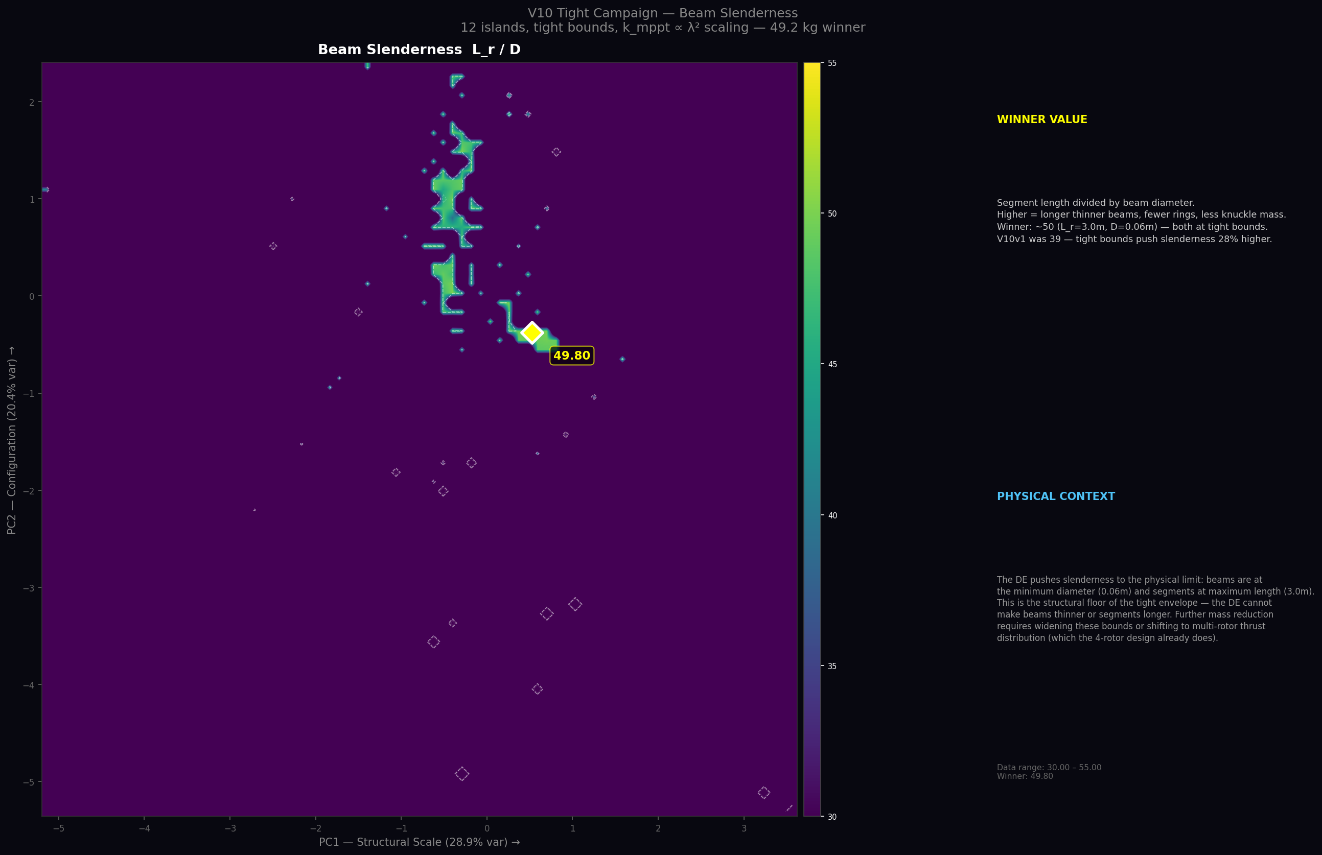
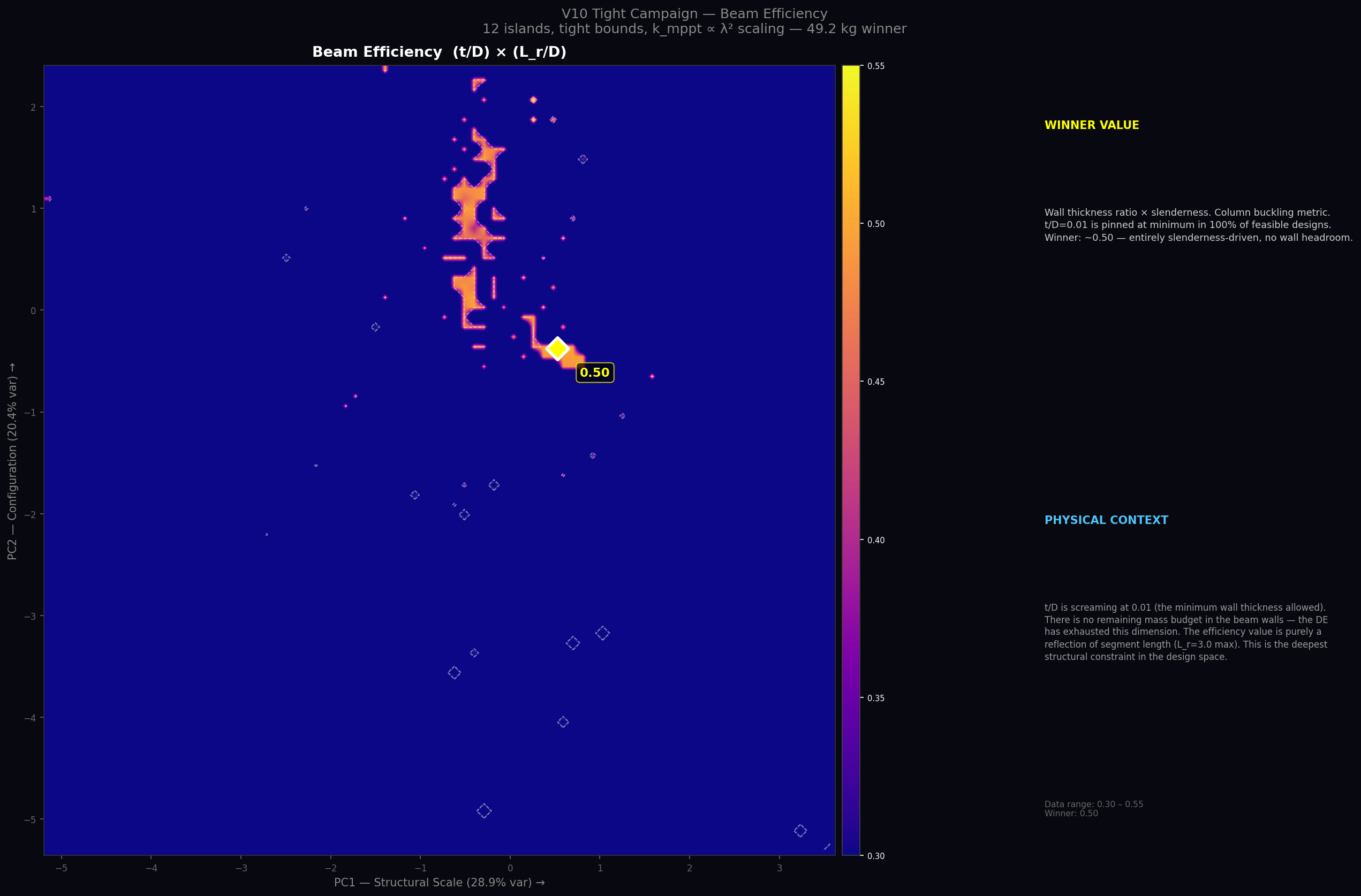
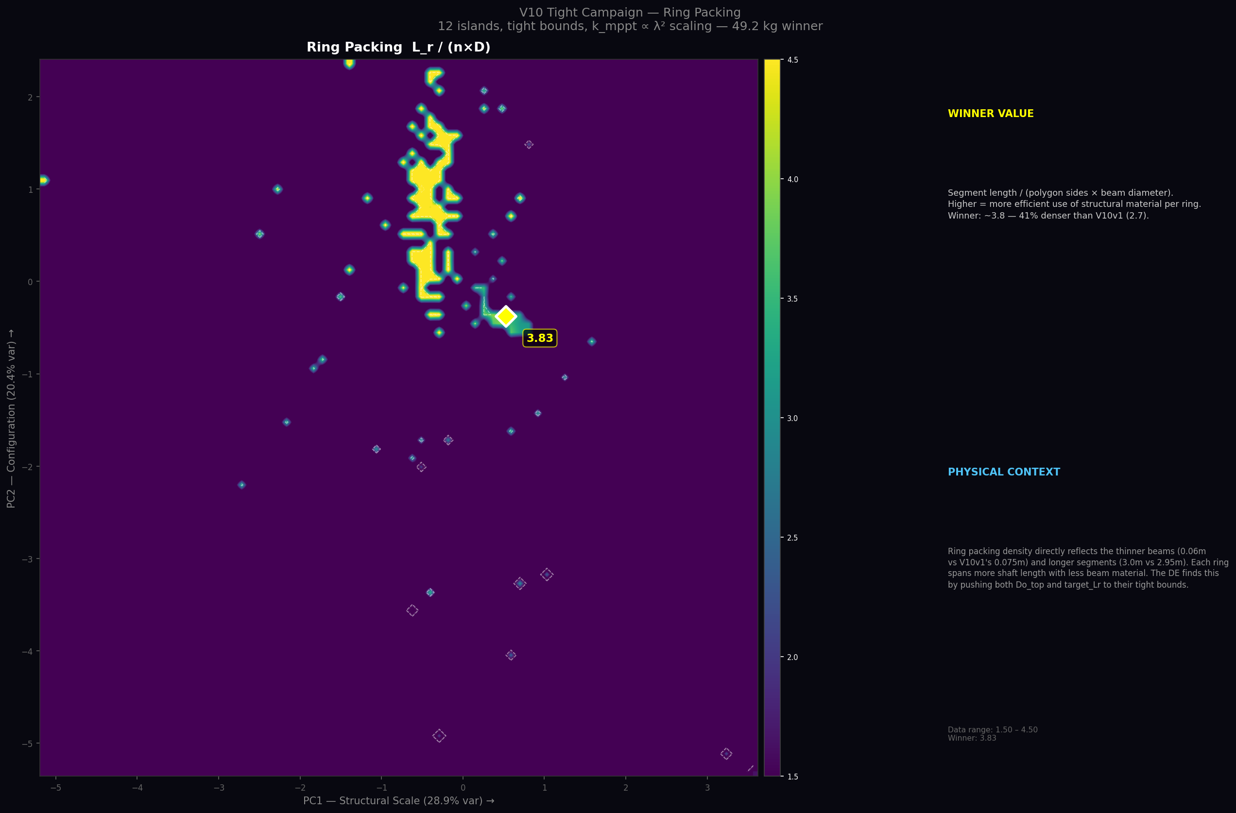
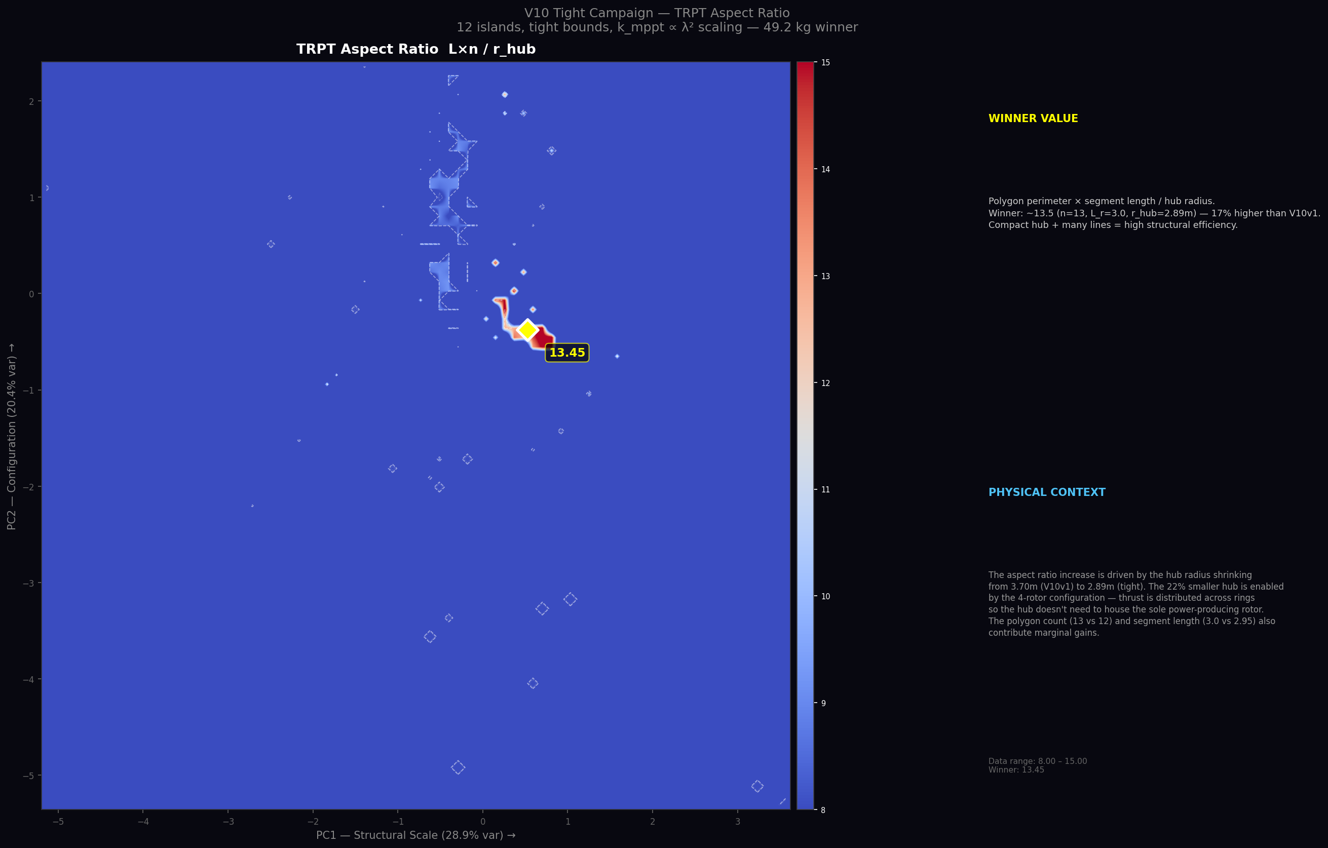
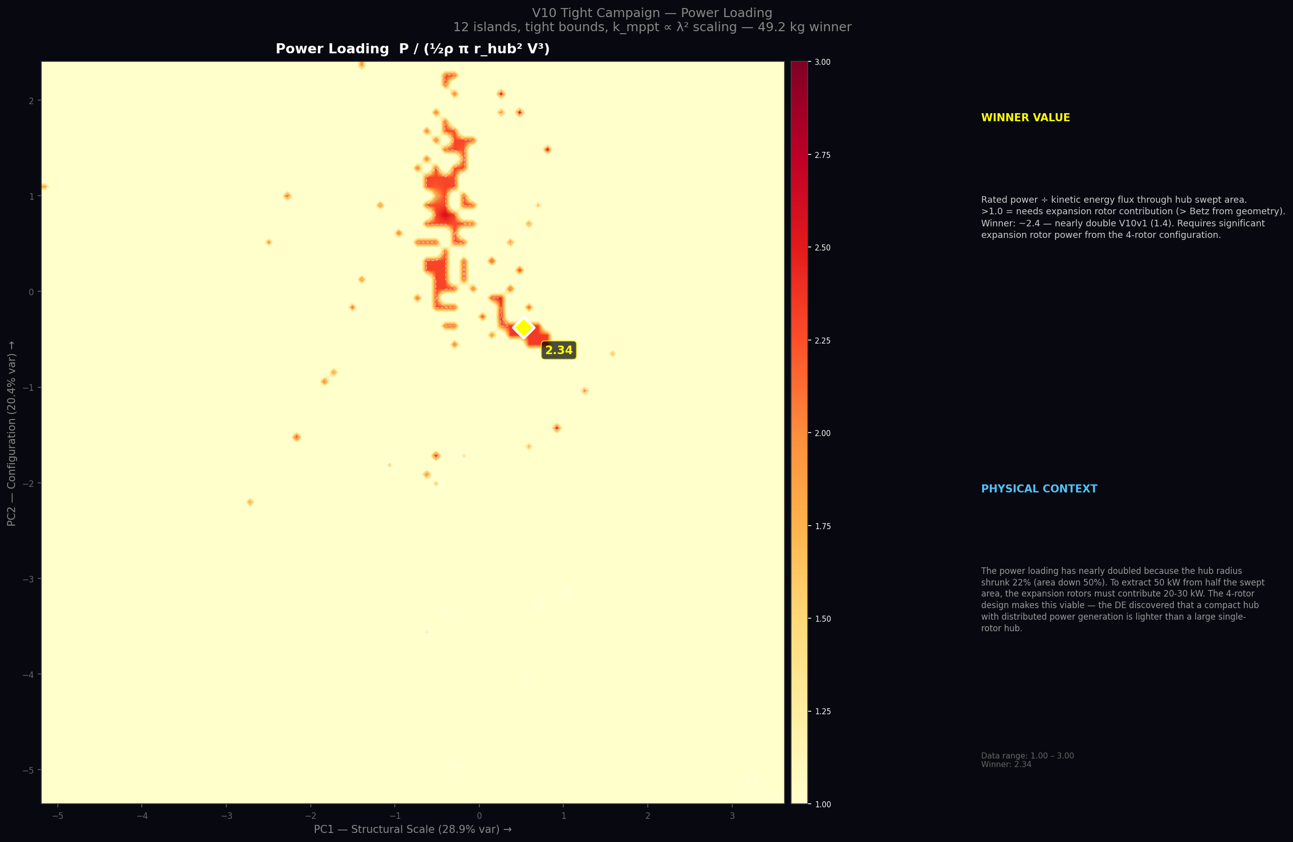
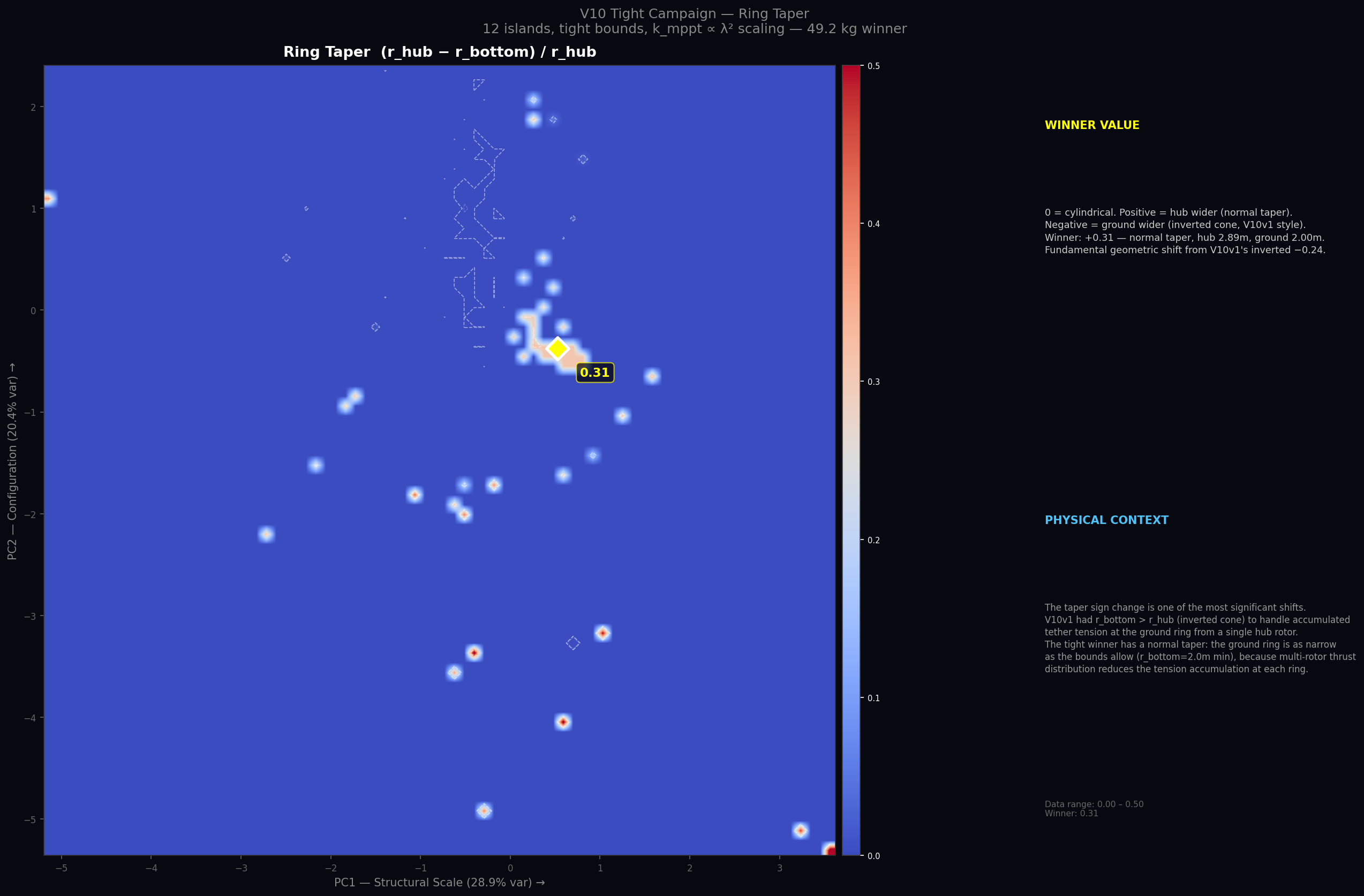
Still some issues with ratio rules and how ring numbers and rotor patterning masks should be connected but … not toooooooooo over crazy
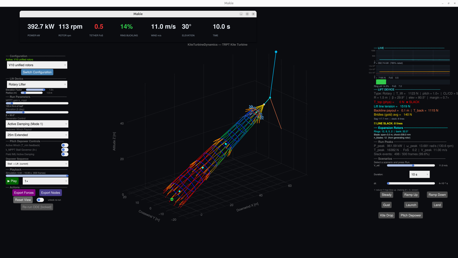
I think I finally have a smooth transmission controller
More testing needed and reports to follow